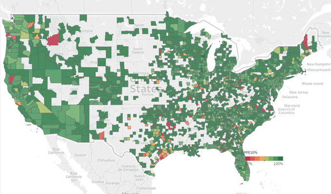
The graphic shows which AVM was tops in each county over the last 8 quarters.
We’ve got the update for Q3 2022. Our top AVM GIF shows the #1 AVM in each county going back 8 quarters. This graphic demonstrates why we never recommend using a single AVM. Again, there are 19 AVMs in the most recent quarter that are “tops” in at least one county!
The expert approach is to use a Model Preference Table® to identify the best AVM in each region. (Actually, our MPT® typically identifies the top 3 AVMs in each county.) Or, you could use a cascade to tap into the best AVM for whatever your application.
This time, the Seattle area and the Los Angeles region stayed light blue, just like the previous quarter. But, most of the populous counties in Northern California changed hands. Sacramento was the exception, but Santa Clara, Alameda, Contra Costa, San Mateo and some smaller counties like Calaveras (which means “skulls”) changed sweaters. Together they account for 6 million northern Californians who just got a new champion AVM.
A number of rural states changed hands almost completely… again. New Mexico, Wyoming, North Dakota, South Dakota, Montana and Nebraska as well as Arkansas, Mississippi, Alabama and rural Georgia crowned different champions for most counties. I could go on.
All that goes to show the importance of using multiple AVMs and getting intelligence on how accurate and precise each AVM is.
We’ve got the update for Q2 2022. Our top AVM GIF shows the #1 AVM in each county going back 8 quarters. This graphic demonstrates why we never recommend using a single AVM. There are 19 AVMs in the most recent quarter that are “tops” in at least one county (one more than in Q1)!
The expert approach is to use a Model Preference Table® to identify the best AVM in each region. (Actually, our MPT® typically identifies the top 3 AVMs in each county.)
One great example is the Seattle area. Over the last two years, you would need seven AVMs to cover the most populous 5 counties of the Seattle environs with the best AVM. What’s more, the King’s County champion AVM has included 3 different AVMs.
A number of rural states changed hands almost completely. New Mexico, Wyoming, North Dakota, South Dakota, Montana and Kansas crowned different champions for most counties.
All that goes to show the importance of using multiple AVMs and getting intelligence on how accurate and precise each AVM is.
Top AVM by county for the last 8 quarters shows a very dynamic market with constant lead changes.
We’ve updated our Top AVM GIF showing the #1 AVM in each county going back 8 quarters. This graphic demonstrates why we never recommend using a single AVM. There are 18 AVMs in the most recent quarter that are “tops” in at least one county!
The expert approach is to use a Model Preference Table to identify the best AVM in each region. (Actually, our MPT® typically identifies the top 3 AVMs in each county.)
Take the Seattle area for example. Over the last two years, you would almost always need two or three AVMs to cover the most populous 5 counties of the Seattle environs with the best AVM. However, it’s not always the same two or three. There are four of them that cycle through the top spots.
Texas is dominated by either Model A, Model P or Model Q. But that domination is really just a reflection of the vast areas of sparsely inhabited counties. The densely populated counties in the triangle from Dallas south along I-35 to San Antonio and then east along I-10 to Houston cycle through different colors every quarter. The bottom line in Texas is that there’s no single model that is best in Texas for more than a quarter, and typically, it would require four or five models to cover the populous counties effectively.
After determining that a transaction or property is suitable for valuation by an Automated Valuation Model (AVM), the first decision one must make is “Which AVM to use?” There are many options – over 20 commercially available AVMs – significantly more than just a few years ago. While cost and hit rate may be considerations, model accuracy is the ultimate goal. A few additional estimates that are off by more than 20 percent can seriously increase costs. Inaccuracy can increase second-looks, cause loans not to close at all or even stimulate defaults down the road.
Which is the best AVM?
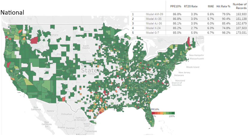
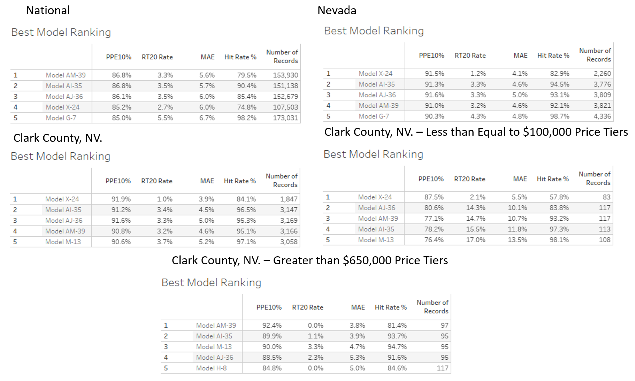
We test the majority of residential models currently available, and in the nationwide test in Figure #1 below, Model AM-39 (not its real name) was the top of the heap. It has the lowest average (absolute) error (MAE) by .1 over the 2nd place model. Model AM-39 is a full percentage point better than the 5th ranked model, which is good, but that’s not everything. Model AM-39 has the highest percentage of estimates within +/- 10% (PPE10%). Model AM-39 has the 2nd lowest percentage of extreme overvaluations (>=20%, or RT20 Rate), an especially bad type of error indicating a significant overvaluation or Right Tailed error.
Figure 1: National AVM Ranking
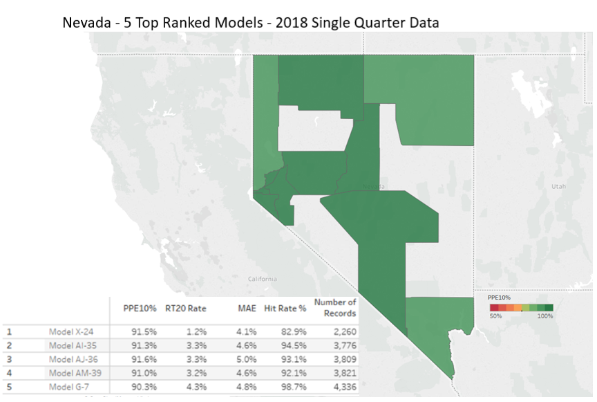
If you were shopping for an AVM, you might think that Model AM-39 is the obvious choice. This model performs at the top of the list in just about every measure, right? Well, not so fast. Consider that those measurements are based on testing AVM’s across the entire nation, and if you are only doing business in certain geographies, you might only care about which model or AVM is most accurate in those areas. Figure 2 shows a ranking of models in Nevada, and if your heart was set on Model AM-39, then you would be relieved to see that it is still in the top 5. And, in fact, it performs even better when limited to the State of Nevada. However, three models outperform Model AM-39, with Model X-24 leading the pack in accuracy (albeit with a lower Hit Rate).
Figure 2 Nevada AVM Rankings
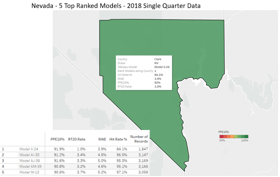
So, now you might be sold on Model X-24, but you might still look a little deeper. If, for example, you were a credit union in Clark County, you might focus on performance there. While Clark County is pretty diverse, it’s quite different from most other counties in Nevada. In this case, Figure 3 shows that the best model is still, Model X-24, and it performs very well at avoiding extreme overvaluations.
Figure 3 Clark County AVM Rankings
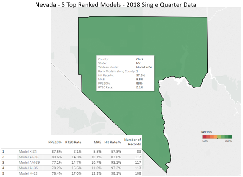
However, if your Clark County Credit Union is focused on entry level home loans with properties values below $100K, you might want to check just that segment of the market. Figure 4 shows that Model X-24 continues to be the best performer in Clark County for this price tier. Note that the other top models, including Model AM-39, show significant weaknesses as their overvaluation tendency climbs into the teens. This is not a slight difference, and it could be important. Model AM-39 is seven times more likely than Model X-24 to overvalue a property by 20%, and those are high-risk errors.
Figure 4 Clark County AVM Rankings, <$100K Price Tier
Look carefully at the model results in Figure 4 and you’ll see that Model X-24, while being the most accurate and precise, has the lowest hit rate. That means that about 40% of the time, it does not return a value estimate. The implication is: you really want a second and a third AVM option.
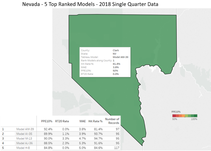
Now let’s consider a different lending pattern for the Clark County credit union. Consider a high value property lending program and look at figure 5, which is an analysis of the over-$650K properties and how the models perform in that price tier. Figure 5 shows that Model X-24 is no longer in the top five models. The best performer in Clark County for this price tier is Model AM-39, with 92% within +/-10% and zero overvaluation error in excess of 20%. The other models in the top five also do a good job of valuing properties in this tier.
Figure 5 Clark County AVM Ranking, >$650K Price Tier
Figure 6 summarizes this exercise, which demonstrates the proper thinking when selecting models. First, focus on the market segment that you do business in – don’t use the model that performs best outside your service area. Second, rather than using a single model, you should use several models prioritized into what we call a “Model Preference Table®” in which models are ranked #1, #2, #3 for every segment of your market. Then, as you need to request an evaluation, the system should call the AVM in the #1 spot, and if it doesn’t get an answer, try the next model(s) if available.
Figure 6 Summary of AVM Rankings
In this way, you get the most competent model for the job. Even though one model will test better overall, it won’t be the best model everywhere and for every property type and price range. In our example, the #1 model in the nation was not the preferred model in every market segment we focused on. If we had focused on another geography or market segment, we almost certainly would have seen a reordering of the rankings and possibly even different models showing up in the top 5. The next quarter’s results might be different as well, because all the models’ developers are constantly recalibrating their algorithms; inputs and conditions are changing, and no one can afford to stand still.
In the AVM world, there is a bit of confusion about what exactly is a “cascade.” It’s time to clear that up. Over the years, the terms “cascade” and “Model Preference Table®” have been used interchangeably, but at AVMetrics, we draw an important distinction that the industry would do well to adopt as a standard.
In the beginning, as AVM users contemplated which of several available models to use, they hit on the idea of starting with the preferred model, and if it failed to return a result, trying a second model, and then a third, etc. This rather obvious sequential logic required a ranking, which was available from testing, and was designed to avoid “value shopping.”[1] More sophisticated users ranked AVMs across many different niches, starting with geographical regions, typically counties. Using a table, models were ranked across all regions, providing the necessary tool to allow a progression from primary AVM to secondary AVM and so on.
We use the term “Model Preference Table” for this straightforward ranking of AVMs, which can actually be fairly sophisticated if they are ranked within niches that include geography, property type and price range.
More sophisticated users realized that just because a model returned a value does not mean that they should use it. Models typically deliver some form of confidence in the estimate, either in the form of a confidence score, reliability grade, a “forecasted standard deviation” (FSD) or similar measure derived through testing processes. Based on these self-measuring outputs from the model, an AVM result can be accepted or rejected (based on testing results) in favor of the next AVM in the Model Preference Table. This application reflects the merger of MPT rankings with decision logic, which in our terminology makes it a “cascade.”
Criteria
AVM
MPT®
Cascade
“Custom” Cascade
Value Estimate
X
X
X
X
AVM Ranking
X
X
X
Logic + Ranking
X
X
Risk Tolerance + Logic + Ranking
X
The final nuance is between a simple cascade and a “custom” cascade. The former simply sets across-the-board risk/confidence limits and rejects value estimates when they fail to meet the standard. For example, the builder of a simple cascade could choose to reject any value estimate with an FSD > 25%. A “custom cascade” integrates the risk tolerances of the organization into the decision logic. That might include lower FSD limits in certain regions or above certain property values, or it might reflect changing appetites for risk based on the application, e.g., HELOC lending decisions vs portfolio marketing applications.
We think that these terms represent significant differences that shouldn’t be ignored or conflated when discussing the application of AVMs.
Lee Kennedy, principal and founder of AVMetrics in 2005, has specialized in collateral valuation, AVM testing and related regulation for over three decades. Over the years, AVMetrics has guided companies through regulatory challenges, helped them meet their AVM validation requirements, and commented on pending regulations. Lee is an author, speaker and expert witness on the testing and use of AVMs. Lee’s conviction is that independent, rigorous validation is the healthiest way to ensure that models serve their business purposes.
[1] OCC 2005-22 (and the 2010 Interagency Appraisal and Evaluation Guidelines) warn against “value shopping” by advising, “If several different valuation tools or AVMs are used for the same property, the institution should adhere to a policy for selecting the most reliable method, rather than the highest value.”