To appreciate what MISMO’s new AVM Common Confidence Score Standard accomplishes, it helps to know where confidence scores have been.
First-generation confidence score schemas were all over the map: 1–10, 1–100, A–B–C–D, High–Medium–Low. In 2005, Doug Gordon, PhD, then chief modeler at Freddie Mac, published a paper called Metrics Matter[i] in an attempt to explain and defend Freddie Mac’s High–Medium–Low schema. That paper ignited a broader industry effort to create a second generation: getting every AVM to calculate and publish a Forecast Standard Deviation (FSD) alongside its value estimate, providing a mathematically grounded and theoretically consistent measure of uncertainty. It was a genuine improvement. Unfortunately, independent testing revealed that not all models were calibrating FSD correctly — their projections did not match actual outcomes.
The AVM Quality Control Standards[ii] rule renewed attention on the problem[iii]. End users still couldn’t reliably compare one model’s confidence output to another’s. That frustration, combined with regulatory momentum, drove the third-generation effort: a truly common confidence score schema with the potential for industry-wide adoption. MISMO’s Common Confidence Score[iv] is that effort. Whether it becomes the enduring standard will depend on what happens next.
“Well Calibrated”
For the first time, there is a shared definition of what a confidence score should mean: the estimated probability that a valuation falls within plus or minus ten percent of the property’s actual market value. Until now, three AVM providers could report confidence scores of “92,” “B,” and “High” for the same property with no way to compare them or hold any of them to a consistent standard.[v] That clarity is genuinely valuable.
But defining what a confidence score should mean is not the same as knowing whether any particular score actually delivers on that definition. The MISMO guidance makes this plain: “for a Common Confidence Score model which is well calibrated, 85% of the AVM values with a Common Confidence Score of .85 will be within 10% of the market value.”
That leaves just one question: how do we know if a model is well calibrated? That is where the real work begins.
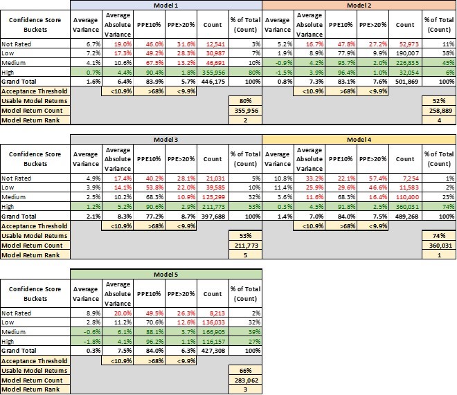
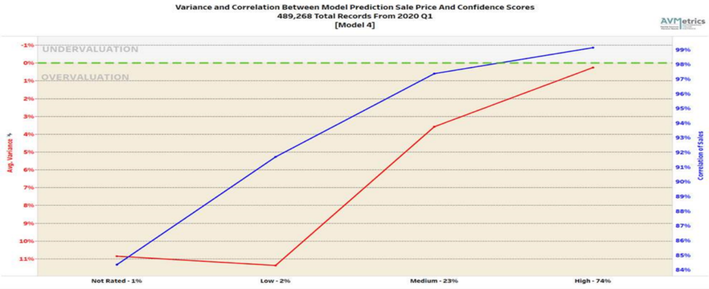
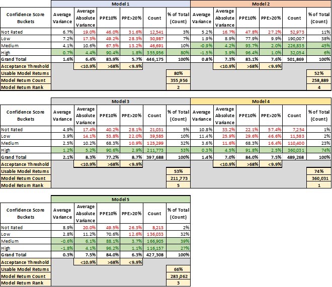
Calibration is distinct from accuracy. A model can produce reasonably accurate values overall while still assigning confidence scores that systematically overstate or understate the probability of being within the expected range. An AVM provider assigning a Common Confidence Score of 0.85 is making a specific, testable claim: that across all valuations carrying that score, roughly 85% should fall within ten percent of true market value. Whether that claim holds is not a matter of definition. It is a matter of evidence — evidence that requires testing.
The MISMO standard acknowledges this directly, noting that the Common Confidence Score “should be subject to regular testing to verify alignment with the above definition.” The standard identifies the need for testing. It does not supply it.
The Scale Problem
Calibration testing is not a simple accuracy check. To verify that a confidence score is well calibrated, you need to observe performance across many thousands of valuations, segmented by score range. You need enough observations in each confidence band to draw statistically meaningful conclusions. Too few data points in the 0.80–0.85 band, for instance, and you cannot determine whether the score is performing as claimed — you are left with approximation rather than verification.[vi]
For most lenders, assembling that volume of test data is genuinely out of reach. Community banks, credit unions, and mid-sized regional lenders may not originate enough loans in a given quarter to support a properly powered calibration test. The only institutions potentially capable of approaching this problem with adequate sample sizes are the largest in the country.
Geography Compounds the Problem
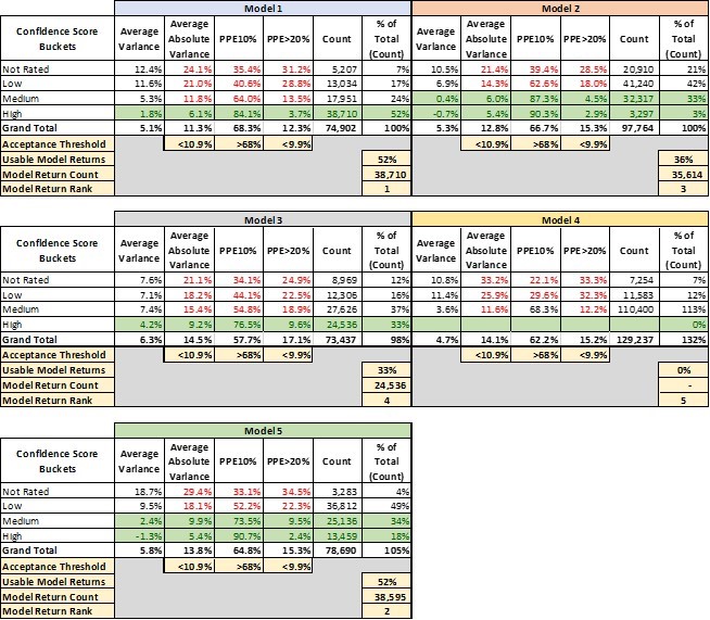
AVM performance is not uniform across geography, and confidence score calibration is no exception. A model that is well calibrated nationally may perform poorly in specific markets — rural counties with low transaction volumes, rapidly appreciating urban submarkets, or areas with heterogeneous housing stock.
A lender operating in those markets needs to know how confidence scores perform there, not just on average. Geographic segmentation requires substantially more data than aggregate testing. Assessing calibration at the county or MSA level requires a dataset large enough to support meaningful analysis in each geography and each score cohort separately — a threshold well beyond the reach of most institutions. A confidence score that performs well nationally but poorly in the counties where a lender does business is not protecting that lender.
Who Verifies the Score?
The MISMO standard represents a voluntary industry commitment to a shared definition. It does not require AVM providers to submit their confidence score models to independent external testing. The verification of calibration is left to the users of those scores — institutions that often lack the data volume and infrastructure to do it rigorously.
This is the structural problem. The models themselves have the ability to test their own confidence scoring, and they certainly do — but they cannot be independent in that assessment. Very few AVM users have the capability to perform that testing. That gap is what independent testing is designed to address.
The AVM Quality Control Standards that took effect in October 2025 require institutions to maintain policies and procedures ensuring a high level of confidence in AVM estimates. Verifying that confidence scores mean what they claim to mean is precisely what that requirement demands.
MISMO has done the work of defining the target. Independently verifying that AVM providers are hitting it — across the full range of markets and conditions on which lenders depend — is the work that follows.
AVMetrics is an independent AVM testing and validation firm serving banks, credit unions, nonbank lenders, and AVM providers. AVMetrics tests AVM performance against actual sale prices across a national dataset of 500,000 to 700,000+ records per quarter, covering 1,700 counties representing 96+% of the U.S. population. Join our community at avmetrics.net to stay up-to-date.
[i] Douglas Gordon, Metrics Matter, The Thomson Corporation and National Mortgage News at 1 (2005).
[ii] Quality Control Standards for Automated Valuation Models, 89 Fed. Reg. 64538 (Aug. 7, 2024), https://www.federalregister.gov/documents/2024/08/07/2024-16197/quality-control-standards-for-automated-valuation-models
[iii] The Appraisal Foundation Industry Advisory Council (IAC) Automated Valuation Model (AVM) Task Force Report, Phase 2: A Report on the Use of AVMs in the Valuation of Residential Real Estate (2023), https://appraisalfoundation.org/pages/resources-b/the-appraisal-foundation-industry-advisory-council-automated-valuation-model-avm-task-force-report-phase-2
[iv] AVM Common Confidence Score Standard & Guidance, Version 1.0 (July 2025), Mortgage Industry Standards Maintenance Organization, Inc. (MISMO).
[v] While AVM providers’ native confidence scores have not been comparable, independent testing methodologies (e.g., AVMetrics’ Predictive Testing Methodology (PTM™)) have provided a consistent, empirically grounded basis for cross-model comparison and validation.
[vi] See William G. Cochran, Sampling Techniques (3rd ed. 1977). Cochran’s formula establishes the minimum sample size required to achieve a desired confidence level and margin of error, underscoring the need for sufficiently large sample sizes within each segmented group.