Hit Rate is a key metric that AVM users care about. After all, if the AVM doesn’t provide a valuation, what’s the point? But savvy users understand that not all hits are created equal. In fact, they might be better off without some of those “hits.”
Every AVM builder provides a “confidence score” along with each valuation. Users often don’t know how much confidence to put in the confidence score, so we did some analysis to clarify just how much confidence is warranted.
In the first quarter of 2020, we grouped hundreds of thousands of AVM valuations from five AVMs by their confidence score ranges. For convenience’s sake, we grouped them into “high,” “medium,” “low” and “fuhgeddaboutit” (aka, “not rated”).[1] And, we analyzed the AVM’s performance against benchmarks in the same time periods. What we found won’t surprise anyone at first glance:
- Better confidence scores were highly correlated with better AVM performance.
- The lower two tiers were not even worth using.
- The majority of valuations are in the top one or two tiers.
However, consider that unsophisticated users might simply use a valuation returned by an AVM regardless of the confidence score. One rationale is that any value estimate is better than nothing, and this is the valuation that is available. Other users may not know how seriously to take the “confidence score;” they may figure that the AVM supplier is simply hedging a bit more on this valuation.[2]
Figure 1 shows the correlation for Model #4 in our test between the predicted price and the actual sales price for each group of model-supplied confidence scores. As you can see, as the confidence score goes up so does the correlation[3] of the model and the accuracy of the prediction as evidenced by the drop in the Average Variance.
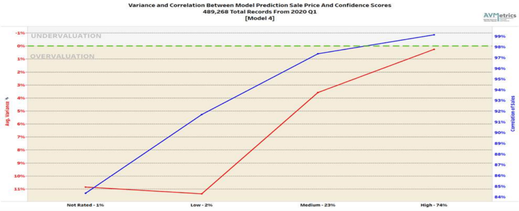
Table 1 lays out 4 key performance metrics for AVMs. They demonstrate markedly different performance for different confidence score buckets. For example, the “high” confidence score bucket for Model 1 performs significantly better in every metric than the other buckets, and what’s more that confidence bucket makes up 80% of the AVM valuations returned by Model 1.
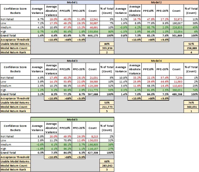
- Avg Variance [4] of 0.7% shows valuations that center very near the benchmarks, whereas lower confidence scores show a strong tendency to overvalue by 4-7%.
- Avg Absolute Variance [5] of 4.4% shows fairly tight (precise) valuations, whereas the other buckets are all double-digits.
- PPE10 [6] of 90% means that 90% of “high” confidence score valuations are within +/- 10%. Other confidence buckets range from 67% to even below 50%.
- PPE>20 [7] measures excessive overvaluations (greater than 20%), which can create very high-risk situations for lenders. In the “high” confidence bucket, they are almost nonexistent at 1.8%, but in other buckets they are 13%, 28% or even 31.6%.
This last metric mentioned is instructive. Model 1 is a very-high-performing AVM. However, in a certain small segment (about 3%), acknowledged by very low confidence scores, the model has a tendency to over-value properties by 20% or more almost one-third of the time.
The good news is that the model warns users of the diminished accuracy of certain estimates, but it’s up to the user to realize when to disregard those valuations. A close look at the table shows that with different models, there are different cut-offs that might be appropriate. Not every user’s risk appetite is the same, but we’ve highlighted certain buckets that might be deemed acceptable.
Model 2 and Model 5, for example, have very different profiles. Whereas Model 1 produced a majority of valuations with a “high” confidence level, Model 2 and Model 5 put very few valuations into that category. “Confidence scores” don’t have a fixed method of calculation that is standardized between Models. It’s possible that Model 2 and Model 5 use their labels more conservatively. That’s one more reason that users should test the models that they use and not simply expect them to perform similarly and use labels consistently.
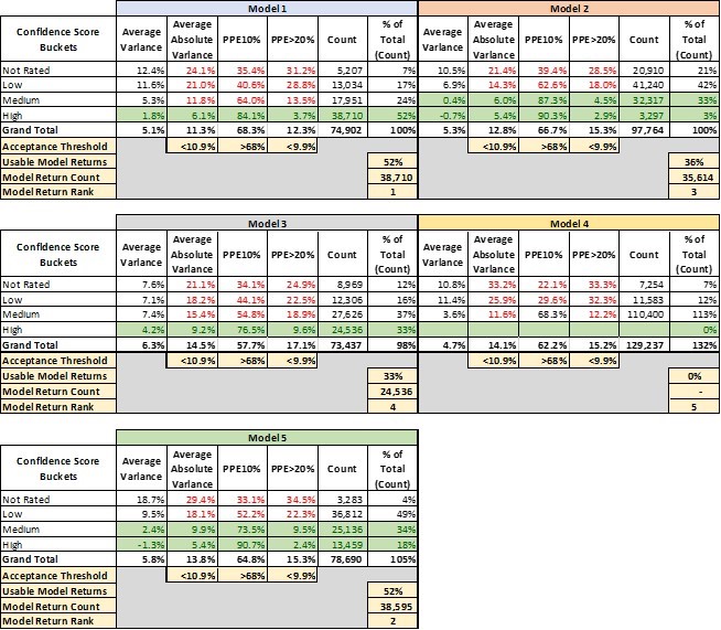
That leads into a third conclusion that leaps out of this analysis. There’s a huge advantage to having access to multiple models and the ability to pick and choose between them. It’s not immediately apparent from this analysis, but these models are not all valuing the same properties with “high” confidence (this will be analyzed in two follow-up papers in this series). Model 4 is our top-ranked model overall. However, as shown in Table 2, there are tens of thousands of benchmarks that Model 4 valued with only “medium” or “low” or even “not rated” confidence but for which Model 1 had “high” confidence valuations.
Different models have strengths in different geographic areas, with different property types or even in different price ranges. The ideal situation is to have several layers of backups, so that if your #1 model struggles with a property and produces a “low” confidence valuation, you have the ability to turn to a second or third model to see if they have a better estimate. This last point is the purpose of Model Preference Tables®. They specify which model ranks first second and third across every geography, property type and price tranche. And, users may find that some models are only valuable as a second or third choice in some regions, but by adding them to the panel, the user can avoid that dismal dilemma: “Do I use this valuation that I expect is awful – what other choice do I have?”
[1] We grouped valuations as follows: <70% were considered “not rated,” 70-80% were considered “low,” 80-90% “medium,” and 90+ “high.”
[2] In fact, this isn’t wrong in some cases. For example, in the case of Model 2, the “medium” and “high” confidence valuations don’t differ significantly.
[3] The correlation coefficient indicates the strength of the relationship between two variables can be found using the following formula:
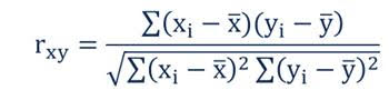
Where:
- rxy – the correlation coefficient of the linear relationship between the variables x and y
- xi – the values of the x-variable in a sample
- x̅ – the mean of the values of the x-variable
- yi – the values of the y-variable in a sample
- ȳ – the mean of the values of the y-variable
[4] Mean Error (ME)
[5] Mean Absolute Error (MAE)
[6] Percentage Predicted Error within +/- 10%
[7] Percentage Predicted Error greater than 20%, aka Right Tail Error